


Overview

Time Series analysis has two main goals:
- Identifying the nature of a sequence of observations.
- Predicting future values using historical observations (also known as forecasting).
In Time Series analysis, it is assumed that the data consists of a systematic pattern, and also random noise that makes the pattern difficult to identify. Most time series analysis techniques use filtering to remove the data noise.
There are two general components of Time series patterns: Trend and Seasonality. The trend is a linear or non-linear component, and does not repeat within the time range. The Seasonality repeats itself in systematic intervals over time. These two components are often both present in real data.
Trend Analysis
Trend analysis is a technique used to identify a trend component in time series data. In many cases data can be approximated by a linear function, but logarithmic, exponential, and polynomial functions can also be used. Dundas Chart for Windows Forms supports polynomial approximation, and also linear approximation - which is implemented as a special case of polynomial approximation.
Regression Analysis
Regression analysis is the study of relationships among variables, and its purpose is to predict, or estimate, the value of one variable from the known values of other variables related to it. Any method of fitting equations to data may be called regression, and these equations are useful for making predictions, and judging the strength of relationships.
Forecasting and extrapolation from present values to future values is not a function of regression analysis. To predict the future, time series analysis is used.
To predict values it is necessary to find a predictive function that will minimize the sum of distances between each of the points, and the predictive function itself. The least-squares method is the most common function amongst the predictive functions, and it calculates the minimum average squared deviations between the points, and the estimated function.
 Note Note |
|---|
| We recommend that you read Using Financial Formulas before proceeding any further. Using Financial Formulas provides a detailed explanation on how to use formulas, and also explains the various options available to you when applying a formula. |
 |
|
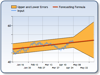
Figure 1: A Forecasting Formula with upper and lower errors (Range chart), as well as the High, Low, and Close prices as a stock chart. |
Applying a Forecasting
All formulas are calculated using the FormulaFinancial method, which accepts the following types of arguments: a formula name; input value(s); output value(s), and parameter(s) that are specific to the type of formula being applied.
Also, before applying the FormulaFinancial method, make sure that all data points have their XValue property set, and that their series' XValueIndexedproperty has been set to false.
The following table indicates what sort of FormulaFinancial method arguments to use when calculating a Forecasting, and also supplies a description of what these parameters mean:
| Parameter |
Value/Description |
Example |
| Formula Name: |
Forecasting
|
FormulaFinancial(FinancialFormula.Forecasting,"2,40,true,true", _ |
| Input Values: |
The values to be used as historical data for Forecasting. |
FormulaFinancial(FinancialFormula.Forecasting,"2,40,true,true", _ |
| Output Value: (optional) |
Value #1: The forecasted values .
Value #3: The lower bound error. |
FormulaFinancial(FinancialFormula.Forecasting,"2,40,true,true", _ |
|
Parameter: |
Parameter #1: Sets a polynomial regression of the specified degree if numeric, but should be the string "Exponential", "Logarithmic", or "Power" to use the other regression types. You can also specify the string "Linear" for the same effect as passing "2".
Parameter #2: Forecasting period (Default: Half of the series length).
Parameter #3: Returns Approximation error (Default: true).
Parameter #4: Returns Forecasting error (Default: true). |
FormulaFinancial(FinancialFormula.Forecasting,"2,40,true,true", _ |
A Line chart is a good choice when displaying the forecasting values, and a Range chart is a good choice for displaying the error bounds.
Financial Interpretation: Forecasting can be used with all Prices to estimate future values, but can also be used with volumes and other indicators.
Calculation: To understand the least-square method let assume that all points (values) which are used as historical data to predict the future belong to the unknown function f(x). The main goal is to find function f(x) which is in many cases almost impossible, or to approximate the f(x) function with another function q(x). Now, if the q(x) function is the polynomial function,
![]()
Formula 1.
the norm, or mean square error, will be a minimum:
Formula 2.
Theorem 1. For each appropriate function f(x), there is a unique least squares polynomial approximation of degree at most n which minimizes Formula 2.
Lets define the function of n+1 variables:
Formula 3.
or
Formula 4.
To find coefficients of the polynomial it is necessary to find a minimum of the function defined in Formula 4.
k=0,1,2,...,n.
Formula 5.
which is equal to:
k=0,1,2,...,n.
Formula 6.
Solving the system of n+1 linear equations we will determine all coefficients defined in polynomial Q(X) (Formula 1.)
Now let's return to our point values and change the function f(x) with pairs of x and y values:
![]()
k=0,1,2,...,n.
Formula 7.
If the n value is equal to 2, the Q(x) polynomial will represent the linear function:
![]()
Formula 8.
The Dundas Chart Forecasting formula returns an array of Y values which represent the results of the Q(x) polynomial function for a determined array of X values. Also there are two more arrays that will be returned by this formula, which represent the upper and lower error boundaries based on two components: standard deviation and the forecasting error.
Example
This example demonstrates how to calculate Forecasting.
| Visual Basic |  Copy Code Copy Code |
|---|---|
| |
| C# | Copy Code |
|---|---|
| |
 See Also
Financial Formulas
Formulas Overview
Using Financial Formulas