Execution and Results
January 2015
support@pureload.com
Execution and Results
|
|
| PureLoad
5.2 January 2015 |
http://www.pureload.com support@pureload.com |
Load execution ca only be started if:
Select the Run->Start Load
Test menu choice or the  button in
the tool bar to start a load execution. The following dialog
window is displayed when the execution is started:
button in
the tool bar to start a load execution. The following dialog
window is displayed when the execution is started:
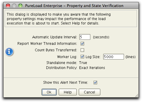
The update interval determines how often results are collected
from the workers. Count bytes transferred must be enabled for
bytes read/write result metrics to be available.
Select the menu choice Run->Stop
Load Test or the  button in the tool
bar to stop the current execution. A dialog is shown where it is
possible to choose if the execution should be stopped gracefully
or aborted brutally:
button in the tool
bar to stop the current execution. A dialog is shown where it is
possible to choose if the execution should be stopped gracefully
or aborted brutally:
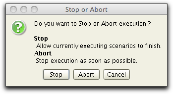
Stop means that all
currently executing scenarios are allowed to finish (the time this
will take depends entirely on the scenarios). Abort will stop execution at
once but it may take some seconds for all results to be reported.
Load executions can be started automatically by defining a start
time. This is convenient when starting a load test late at night
without actually monitor the execution.
Select the menu choice Run->Run
Load
Test at... to display a dialog to schedule a start time.
Note that when a delayed start has been scheduled, this will be
indicated in the status bar displaying Waiting... To cancel a delayed load execution
that are waiting to be started, select the Run->Start Load Test at...
menu choice and then select the Stop
Timer button
The distribution of the scenarios in a load test can be updated
while the test is running by using the menu choice Run->Update Distribution.
This will update the distribution of the scenarios in a running
load test with the values in the Scenario Editor. After updating
the load test progress bar may no longer be accurate, but the test
will be executed according to the new distribution until finished.
Note that only the distribution details will be updated - any
other changes in the scenarios will be ignored. The scenario structure may not be changed
between starting a load test and using Update Distribution. Doing
so will give unexpected results.
If Worker persistence is enabled using Tool Properties,
results are stored on the worker side. This means that after an
execution is finished, the Run->Get
Persistent Results menu choice may be used to retrieve
the last saved results.
When persistent results are fetched, the console will retrieve the
results and update most result information as when used in
real-time.
This option may typically be used when running for a long time,
where you want to check results after execution is finished.
The following explains the various information and metrics
reported in PureLoad and how to interpret them.
The name of all tasks as they appear in the result presentation
are the same name as specified in each tasks Name parameter. This
identifier is used to group tasks in the result presentation.
The Time field in the status bar indicates in hours, minutes and
seconds the elapsed time of the load execution. This timer starts
when the first task is starting to execute. The timer stops at the
same time as the last task in the actual scenarios has finished
executing.
The following general metrics exists:
Result metrics that include results for Scenario and Task
Sequences objects are summaries of the contained child objects.
Metrics reporting time might report N/A which indicates a Not
Applicable result. This might be a result of a scenario with only
failed tasks. In this case it is not possible to calculate the
time for Min, Average, etc. All time metrics are always expressed
in seconds and milliseconds. These are separated using the
character for the actual locale.
The Tasks/Sec needs some extra attention since its reported
values might confuse the results of the load execution. In the
Summary view there is a column indicating Tasks/Sec which is also
Scenario/Seq and Task Sequences/Sec depending of what is in the
summary table.
It is, independently of what object type it represents, calculated
by dividing the total execution time of the executed objects with
the total time of the load execution.
Some tasks have the ability to report bytes transferred between
the task and the tested application. For these the following
metrics are reported:
In addition Time To First Bytes (TTFB) is reported by
HTTP based tasks. TTFB is the duration from making an HTTP request
to the first byte of the page being received. This time is made up
of the socket connection time (if no previous connection), the
time taken to send the HTTP request, and the time taken to get the
first byte of the page.
The results main tab presents various result metrics from a load
execution that is either executing or has finished. The results
information is updated on a regular basis during a load execution,
using the update interval as specified in the Tool Properties
dialog.
The results main tab contains several views organized in sub tabs
at the bottom of the screen:

The Summary View shows all result metrics for the selected node
in the worker tree to the left in the view. Selecting the Naming
node in the tree will show the complete summary for all scenarios
that are included in the load execution independently on which
host that were executed. The summary can be narrowed by selecting
a Manager, Worker or Worker Thread node in the tree, i.e.
selecting a Manager node will show the result summary based on
what all workers and worker threads for that manager have
executed. Selecting a specific Worker Thread will only show the
result summary executed by that worker thread.
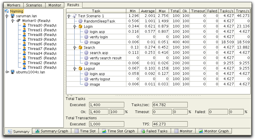
The figure above shows the summary information for a load
execution that has completed with a detailed scenario tree and an
overall summary. This load test included one scenario, Test
Scenario 1, that was executed for 100 iterations. The worker tree
lists all worker threads that were part of the execution.
Selecting a node in the tree will list the summary for that node
and all children. This example illustrates the Naming node and
thereby will the summary information list the metrics for all
worker threads.
Execution times minimum, average and maximum are shown in seconds. The minimum value for the Login sub sequence above is 0.344 s. This is not the sum of the tasks: 0.316 s + 0 s + 0.006 s = 0.322 s. The minimum time executing Login was never lower than 0.344 s. The individual task times 0.316, 0 and 0.006 come from different executions of the sequence. (The same applies to scenario nodes.) Tasks which does not report any result are not included in the aggregated sequence result. This means that the real-world execution time of a scenario may be longer than the scenario average time multiplied by number of executions. Tasks / second is calculated using number of executions divided by real-world execution time.
Note that some of the tasks has been executed more than 100 times
even though the Iteration setting for all tasks were set to 1
during editing of the scenario. The reason for this is that tasks
with the same Name in a path will be reported as one task. An
example is the Test
Scenario/Login/image task, that includes 4 tasks, both
named image.
Also note that there is a distinction between number of executed
Tasks and number of executed Transactions. Number of executed
tasks is all tasks that reported a result. Some tasks also report
transactions. For example HttpGetTask reports 1 transaction when
successfully executed, but RandomSleepTask does not report any
transaction.
The Summary Graph is basically the same as the Summary view but
presented in a bar graph. Here you select the actual scenario
objects to be presented in the graph.
This graph is typically useful to get an overall understanding of
what requests that takes more time to execute compared to others.
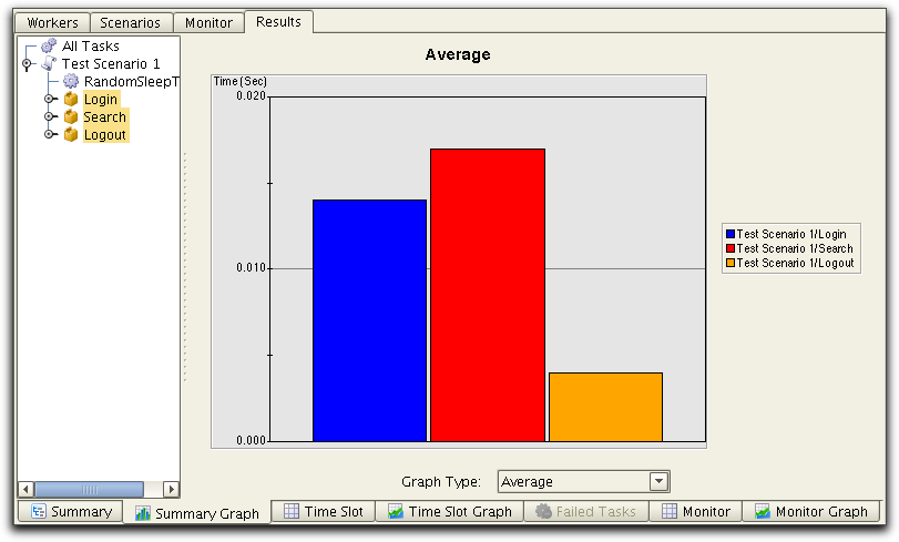
The figure above shows the average execution time for the
selected task sequences. Select any nodes in the scenario tree to
show them accordingly in the graph. The order of the bars (and
legend) in the graph will be the same as the order each node in
the scenario tree is selected.
The Graph Type box is
used to set what metrics to show in the graph.
The Time Slot tab shows metrics in a tabular format. There is one
row per update interval (time slot) in the table. The first column
shows the actual time for the time slot. All other columns shows
metrics for the selection(s) made in the scenario tree.
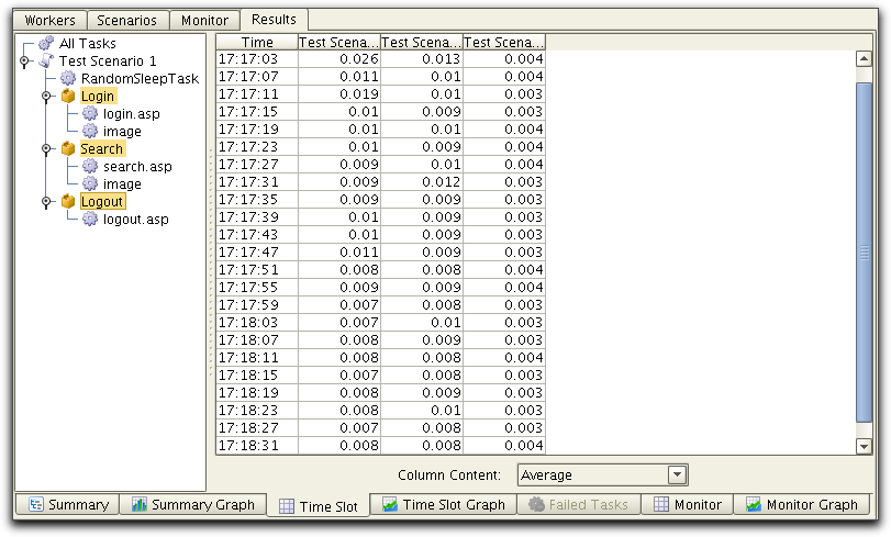
In this example we have chosen to show the Average metrics.
There might be empty slots in the table and this indicate that
there were no results reported during that period. This might also
indicate that the value of update interval seconds should be
increased.
The Time Slot Graph shows the same information as the Time Slot table, but in a line graph view.
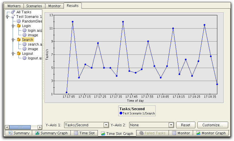
Again use the box below the graph to set what metric to show in
the graph. It is also possible to zoom the graph on the X-axis by
selecting the area in the graph using the mouse. Use Reset to
return to the original zooming.
In addition, this view allows for two metrics to be displayed.
Select a 2nd metrics using Y-Axis
2 to display second metrics:
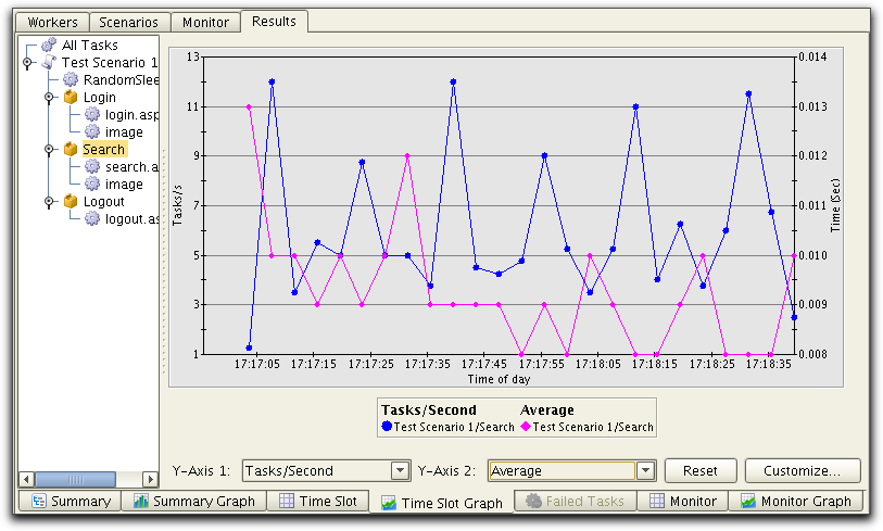
Here we display Task/Second (left Y-axis) and Average (right
Y-axis).
It is also possible to zoom the graph by selecting the area in
the graph using the mouse. Use Reset to return to the original
zooming.
Detailed task results for failed Tasks can be viewed in the
Failed Tasks sub tab.
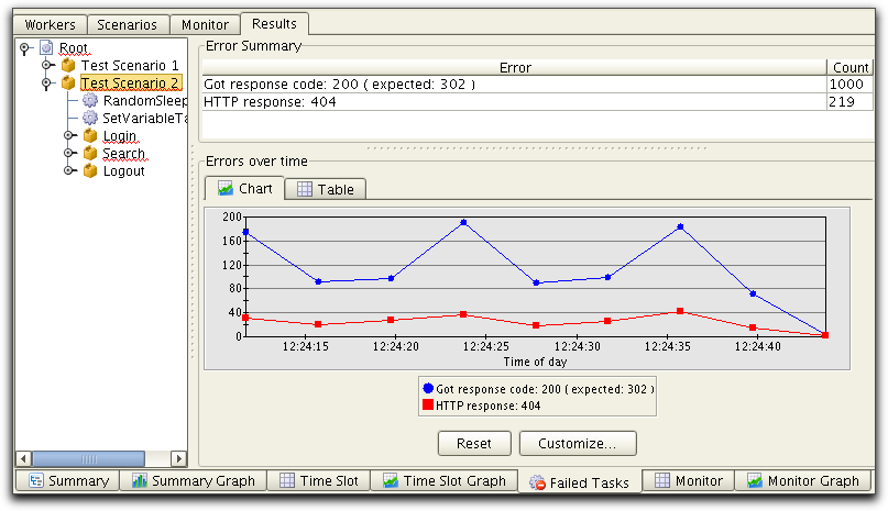
The scenario task tree shows all executed scenarios, where
scenarios with errors are underlined with a red line.The view to
the right shows a summary table of the various reported errors and
a graph with errors over the execution time.
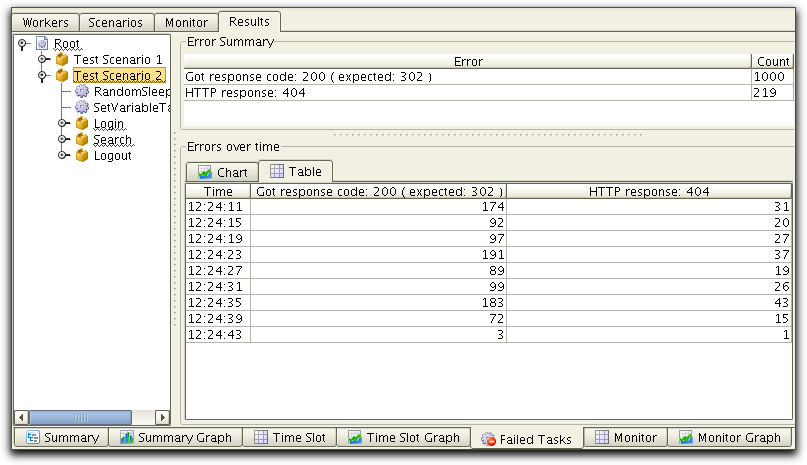
The reported error over time can also be viewed in table format,
by selecting the Table tab.
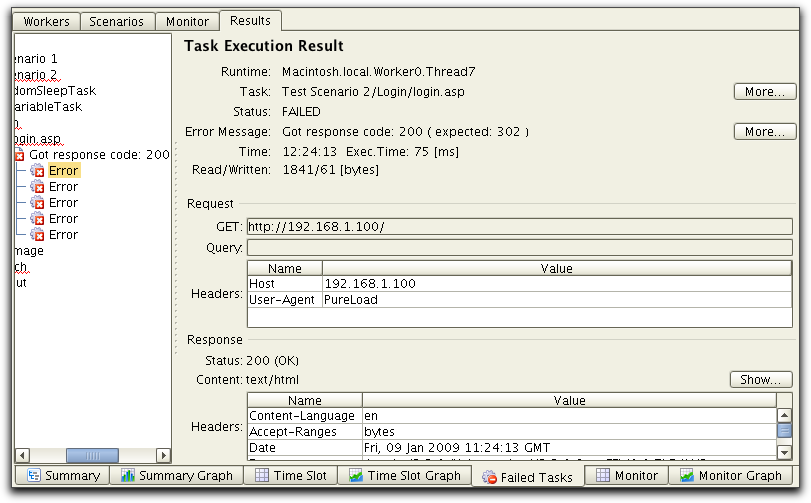
To see more errors expand the tree down to where the individual
errors are displayed. Select a child error node to see details
about a reported error:
To reload the view, select a node in the tree and choose the View->Reload menu option or
the  in the tool bar. Reloading error
information and fetching detailed error nodes might take some time
to process, which will be indicated in the user interface.
in the tool bar. Reloading error
information and fetching detailed error nodes might take some time
to process, which will be indicated in the user interface.
Results from execution of defined server monitors, in table
format, can be viewed using the Monitor tab.
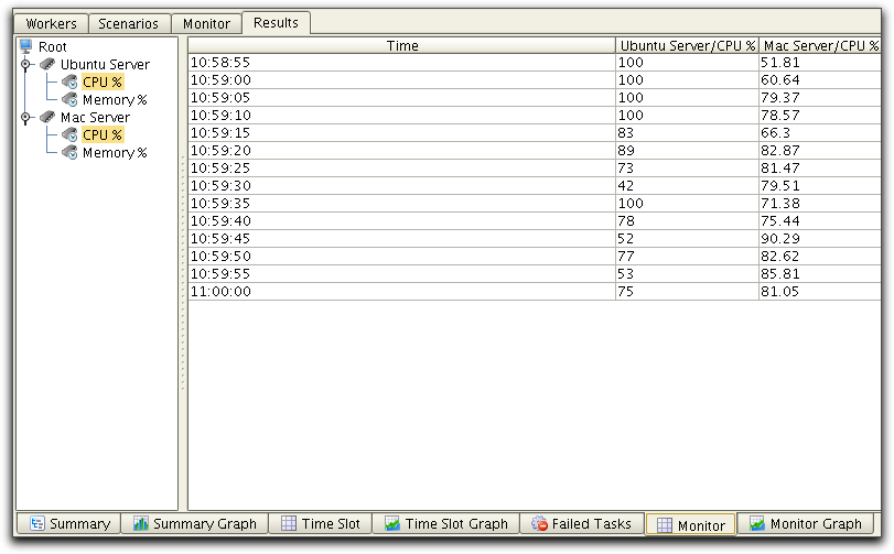
Select the resources in the tree to the left that you want to
include in the table.
To see results from execution of defined server monitors, in graph view, select the Monitor tab.
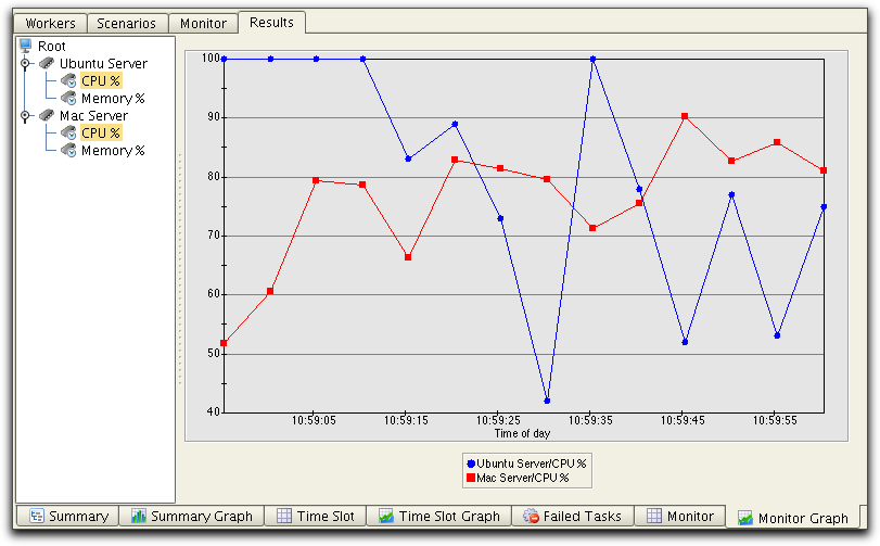
Select the resources in the tree to the left that you want to
include in the graph.
The File->Export menu
option is used to export a snapshot of the current visible result
view into a file.
The tables in the Summary
and Time Slot views are
exported in CSV (Character Separated Values) format. The column
separator and the new line character that will be part of the
exported file can be set in the tool properties.
Tip: It is also possible to copy
cells in any of the result tables to the system clipboard for
later inclusion into for example a spreadsheet program or
similar. Do this by selecting cells in the actual table and then
press Ctrl-C for copy.
Now open the target document and paste the cells into it. The
column and new line separators are specified in tool properties.
The graphs in Summary Graph
and Time Slot Graph views
are exported as PNG (Portable Network Graphics) files.
Information from the Summary
and Time Slot views, as
well as comparer data can also be exported using the File->Export All menu
option. This will display an Export
Wizard, described later in this section.
The report functionality is accessed by the File->Generate Report menu
choice or the  button in the tool bar.
The content of the generated report can be configured in many
ways. Since it is HTML and PNG image files that are produced the
report may be viewed in the majority of web browsers.
Configuration of the report is controlled using the report
wizard. The first pane displayed are:
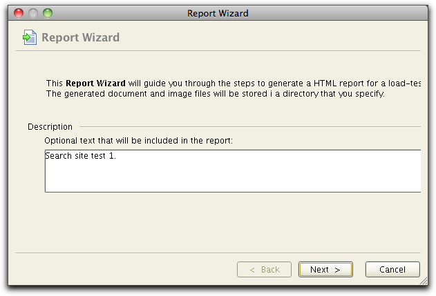
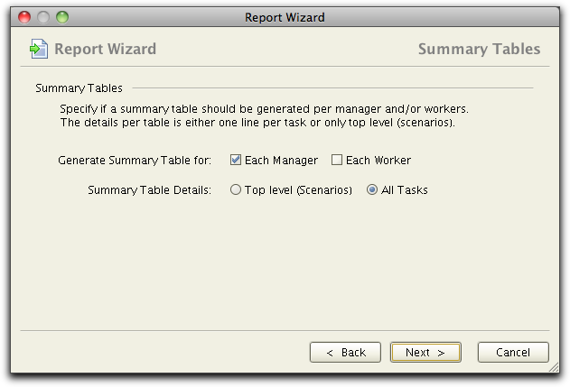
Here you specify any text you want to include in the report. The
next pane allows you to select how detailed the summary tables to
be and if you want a summary per manager and/or worker.
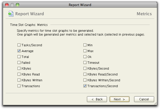
Then you can select which tasks to generate time slot graphs for:
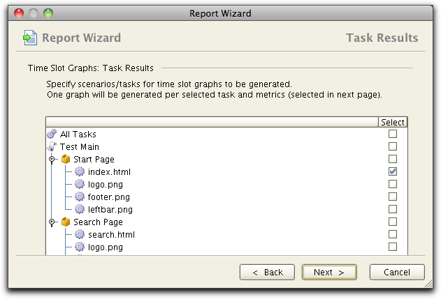
For the selcted task, one graph will be generated for each metric
selected:
Finally you specify where the generated report and image files
will be stored and the name of the report HTML document:
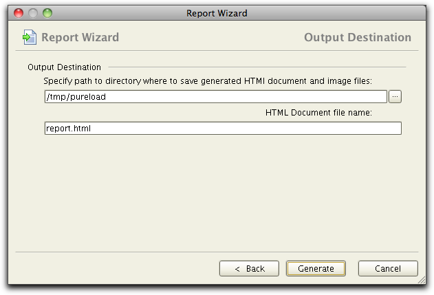
By selectin the Generate button the report is genarated. When
done you will be presented with a choice to directly display the
document in a browser.
Exporting the results of a load execution allows using the use of the Result Comparer tool. This tool is used to visualize the results of several load tests and to compare results. Typical usage is when when performance enhancements has been applied in the server application between load tests.
To export comparer data use the File->Export
Comparer Data menu option. A dialog will be presented too
choose where to save the comparer data file.
Use the File->Export All menu option to display the Export Wizard where you can select to export data from the Summary and Time Slot views, as well as comparer data:
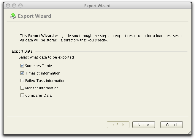
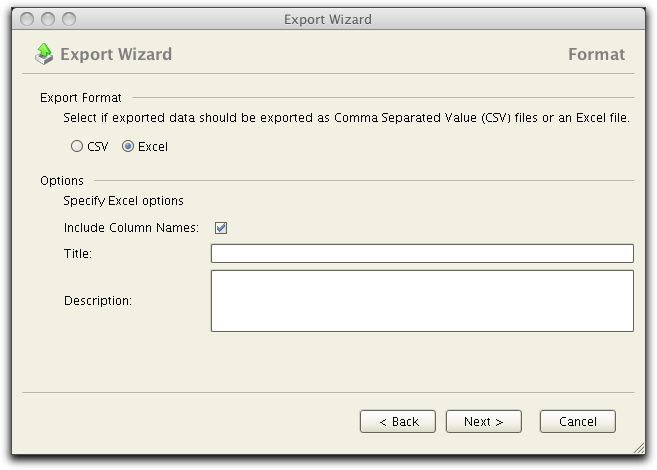
The Export Wizard will guide you through a set of panes to configure what to be exported, depending on what data you choose to export. When using the export wizard you also have a choice to export summary information and time slot information in Excel format at well as CSV format:
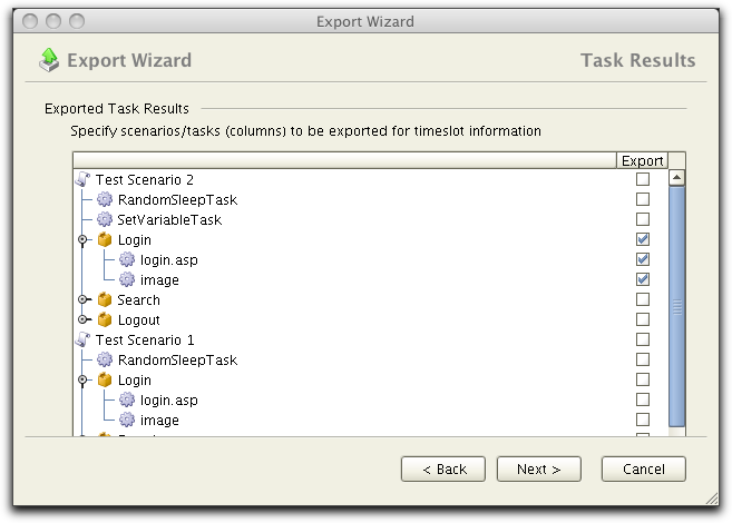
It is possible to specify which parts of the scenario results that
should be included in the exported data:
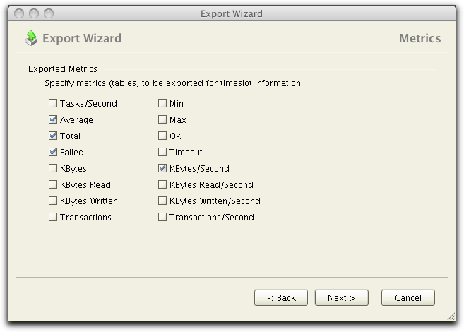
The metrics to include can be chosen individually as well:
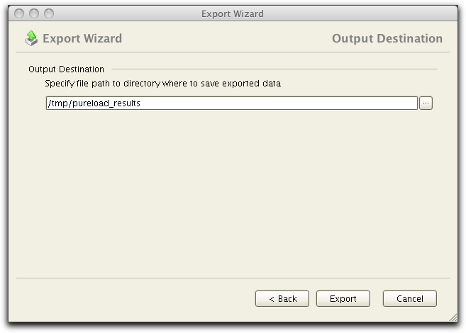
Finally a pane to select a directory where the exported data
files to be saved is presented.